The six pillars

These six are what the work is. The next six pages introduce each pillar in one breath. Then we go in.

Savanna

A ternary lattice running on Apple Silicon GPU, scheduling cells in seven phases via distance-2 chromatic separation on a hexagonal grid. The substrate that hits the central GCUPS number on a laptop.

Read more: Savanna Engine repo · Savanna white paper · 7-coloring explained — interactive

DagDB

Every node holds a 64-bit truth table — six inputs, one output, the same primitive that lives at the heart of an FPGA. Nodes wired into a ranked acyclic graph; the engine evaluates the whole graph in parallel on the GPU each tick. Snapshots, write-ahead log, multi-version reads — durable like a real database.

The BACK_EDGE primitive lets state latch across tick boundaries — unlocks AC-3 constraint propagation, Hopfield-style recurrent networks, Boolean networks with feedback.

Read more: DagDB repo · DagDB white paper · Engine site · SQL architecture

Proteins

Geometric reasoning over protein conformations. Substrate, not folding prediction. AlphaFold gives you the structure; we operate on it.

The hepatocyte 10⁷ Pass 2 schema lays in a spatial-adjacency layer with hepatic-zonation policy ranks (sixteen levels, periportal to pericentral). The graph encodes what is adjacent in space; the engine reasons over the topology.

Read more: Isomorphic Walk repo

Applied Math

Memory layout via Morton Z-curve — cache-friendly traversal that delivers a 2.11× speedup over row-major at one billion cells. Distance-2 chromatic separation on the hexagonal grid uses exactly seven colours (Molloy–Salavatipour 2005), with the engine using (col + row + 4·(col & 1)) mod 7 as the colour-class formula. The combination is what makes the substrate parallelizable on commodity GPU hardware.

Read more: Savanna Morton charts · 7-coloring explained

Architecture

Apple unified memory used as zero-copy substrate — no CPU/GPU buffer boundary. Tile-streaming scaffold for 10¹¹ nodes on one M5 Max: page tiles to and from NVMe, two tiles resident at a time, cross-tile addressing via 24-bit-tile + 40-bit-local u64 global ID.

Three-environment separation — dev / test / prod under guarded paths. Triple-write to markdown, DagDB, and Postgres with markdown as the leader.

Read more: DagDB engine repo · DagDB white paper

Theoretical Math

The substrate the simulation engines run on assumes regularity properties of the underlying space. CVPDE-class results — Almgren-monotonicity-style — are foundation lemmas that have to hold for the substrate to behave the way the engineering claims.

Open directions: extension to non-uniform grids, generalization beyond hexagonal lattices, sharper bounds on the chromatic number under non-uniform-distance constraints.

Read more: DagDB engine repo

Direction 4 — Savanna Engine (existence proof for the scale path)

Calibration: this slide reports a VERIFIED build. Savanna ran 100 billion cells over 9 hours on one M5 Max laptop, peaked 15.8 GCUPS, wrote 500 GB of state to disk. Same dispatch + Morton + 7-coloring machinery DagDB inherits — making this the existence proof for DagDB’s trillion-cell scale path. Honest framing guard: Savanna’s FLUID kernels (scent, density, predator-prey, peristaltic streaming) are intentionally NOT in DagDB. Conflating the two is overclaim risk. See one_pager.md’s “DagDB inherits Savanna’s physics engine” overclaim callout for the precise lineage boundary.

What

A predator-prey-grass spatial-lattice simulator on Apple Metal GPU, running discrete biology on a 1024×1024 hex grid as a test workload for the underlying spatial-compute machinery. The biology is the load — the engine is what’s being measured.

Three engineering primitives load-bearing the throughput:

• Hex 7-coloring for lock-free parallelism. Distance-2 chromatic number of the squared hex lattice is 7 (Molloy & Salavatipour 2005); same-coloured cells share no neighbour, so each colour group dispatches in full GPU parallelism with no atomics.
• Morton Z-curve memory layout — 2.11× speed-up at 1 billion cells over row-major, pure L2-cache-locality win on UMA hardware.
• Lock-free chromatic dispatch — 13 kernel dispatches per tick, state lives in unified memory, zero CPU↔︎GPU copy.

Same machinery DagDB inherits (HexGrid, Carlos Delta encoder, halo file format). Different per-cell state: Savanna stores fluid + scent + entity tables; DagDB stores Boolean LUT6 + ranked DAG metadata.

Why on the the deck

Existence proof for the trillion-cell scale path. The verified 100 B / 9 h Savanna run on one M5 Max laptop is the highest scale the substrate machinery has actually shipped. DagDB’s tile-streaming spec for 10¹¹ nodes (docs/tiled-streaming.md) targets the same hardware envelope. Without Savanna’s existence proof, DagDB’s trillion-cell goal is just a target. With it, the engineering question reduces to “can we tile the LUT6 / BACK_EDGE state across NVMe at the same machinery’s throughput envelope?” — a tractable engineering question rather tha feasibility one.

Numbers (verified, M5 Max, 10-run validated)

• 100 B run hit M5 thermal ceiling; 9-hour wall reflects sustained throttled state, not headroom. Same dispatch machinery, different per-cell load.

Peak: 27.1 GCUPS measured at 16 M cells, 10-run validated, < 1 % standard deviation. Sustained 100 B: 15.8 GCUPS — figure cited on the deck.

One representative engineering overcome — Type II satiation

Saw the predator-prey simulation collapse repeatedly to extinction: lions kill all zebras, then starve. Classic thermodynamic suicide switch. Gemini Deep Think’s diagnosis: the per-tick lion energy update needed a satiation cap so well-fed lions stop hunting and become a “physical meat shield” — preventing the runaway overhunting that triggered the death spiral.

Implementation: one inequality in the lion tick_phase kernel (if my_energy >= SATIATION_THRESH: don't_hunt). Predator-prey populations stabilize at oscillating limits. Same fix Holling 1959 prescribes for ODE-level Lotka-Volterra; we just learned why it’s load-bearing on a discrete lattice the hard way.

The white paper’s eight-overcome teardown lists the full set — including the LCG-parity “ghost wind” hash bug, the chromatic- advection dispatch-order drift, the Atto-Fox sub-individual extinction trap, and the Voronoi-formation “lion haboob” that emerged unbidden from the corrected dynamics.

Pointers

• White paper: https://norayr-m.github.io/savanna-engine/whitepaper.html — full eight-overcome teardown + benchmark methodology + ablations
• Repository: https://github.com/norayr-m/savanna-engine
• DagDB lineage tracking: dagdb/Sources/DagDB/HexGrid.swift (lifted verbatim), Sources/DagDB/CarlosDelta.swift (encoder preserved). Per-cell state and biology kernels NOT inherited.

Calibration block

Honest framing footer

What’s not claimed. Savanna is a fluid-dynamics-capable spatial lattice engine — scent diffusion, peristaltic streaming, predator- prey kinetics. DagDB is not. The lineage between them is dispatch patterns + halo file format + Morton + 7-coloring. The fluid / scent / density kernels were intentionally dropped when DagDB became Boolean-LUT-only. Conflating the two = the precise overclaim risk flagged in one_pager.md. The existence proof Savanna provides for the scale envelope is real; the engineering question for DagDB at 10¹² is “can we tile LUT6 + BACK_EDGE state across NVMe at this throughput envelope” — which is a tractable port, not a feasibility claim.

Filled by slvr 2026-05-01. Pub-screen gate before commit to assets.

Direction 5 — DagDB Engine

Owner: dag (engine internals); pub (editorial pass) Status: DRAFT 1 (2026-05-02) Tier: 2 (medium level / main directions) Calibration anchor: ../one_pager.md

Slot scope

One-slide condensation of DagDB’s engine story, sized for the architect-grade audience to grasp the engine class and what makes it different.

Required content: - Headline: graph database where every node is a 64-bit truth table (LUT6); ranked DAG, evaluated on the GPU each tick - BACK_EDGE primitive (synchronous-circuit register pattern) verified via AC-3 round-trip — VERIFIED, 120+ Swift tests green - Snapshot v4 + WAL + MVCC — durable like a real database - Bitwise LUT composition (COMPOSE AND/OR/XOR/NOT) for runtime graph simplification - ~2 ms per tick at 1 M nodes on M5 Max (engine throughput at the demo scale) - Pointer to the engine repo + the wiki tab at github.com/norayr-m/dagdb-engine/wiki

What this slide does NOT do: - Claim “thinking engine” — explicitly off per one_pager.md. Speedboat for one narrow class of structured-dependency reasoning. - Mix Savanna-physics framing in (those are different engines)

Slide content (narration-ready)

Headline. A graph database where every node holds a 64-bit truth table — i.e., a programmable Boolean function with up to six inputs. Same primitive that lives at the heart of an FPGA. Nodes wire into a ranked acyclic graph; the engine evaluates the whole graph in parallel on the GPU each tick. Persistent like a real database — snapshots, write-ahead log, multi-version reads. One machine.

The four verified pieces.

1. 6-bounded ranked DAG with LUT6. The engine. Bounded fan-in keeps per-node compute trivial; the rank invariant (rank(src) > rank(dst)) makes topological order well-defined; LUT6 means each gate is one indirect read of a 64-bit integer.
2. BACK_EDGE primitive — synchronous-circuit register pattern. Combinational logic for the within-tick pass, plus typed back-edges that latch state across tick boundaries. The same shape as Verilog reg / non-blocking assignments. Verified end-to-end by AC-3 Australia 3-coloring round-trip against an independent Python reference: per-tick equality across 21 register nodes, converges in 2 synchronous ticks. 120+ Swift tests green. Without BACK_EDGE the substrate hosts only feed-forward Boolean DAGs; with it, AC-style constraint propagation, Hopfield-shape recurrent networks, and any register-clocked dynamical system become natively expressible.
3. Snapshot v4 + WAL + MVCC. Power-loss-durable writes via F_FULLFSYNC + replaceItemAt + dir fsync (Apple-SSD discipline). WAL replay rolls forward through a crash. Reader sessions take snapshots without blocking writers — concurrent queries see a consistent view of the graph.
4. Bitwise LUT composition (COMPOSE). COMPOSE AND src1 src2 INTO dst, plus OR/XOR/NOT. Collapses subgraphs into single LUTs without re-evaluating the original tree at runtime. Useful for graph simplification passes and for synthesizing complex gates from primitives.

Throughput. ~2 ms per tick at one million nodes on M5 Max.

Diagram — full architecture

Lifted verbatim from dagdb-engine/site/sql-architecture.html (slide 15).

Surface. Engine repo github.com/norayr-m/dagdb-engine, wiki tab on the same repo, browser-runnable demos at norayr-m.github.io/dagdb-engine/site/. The BACK_EDGE wiki page is the deepest written reference for the primitive.

Source material

• BACK_EDGE wiki page: https://github.com/norayr-m/dagdb-engine/wiki/Back-edges
• Engine README: https://github.com/norayr-m/dagdb-engine
• Engine site: https://norayr-m.github.io/dagdb-engine/site/index.html
• Calibration rows in ../one_pager.md: BACK_EDGE/AC-3, Snapshot v4, MVCC, COMPOSE LUT — all VERIFIED

Calibration block (fill at draft time)

Honest framing footer (template)

What’s not claimed. DagDB is not a general thinking engine. Missing: variables, quantifiers, first-order logic, probabilistic truth, search/planning, recursive within-tick evaluation. It is a fast specialised substrate for one class of structured-dependency reasoning.

Stubbed by Pub on 2026-05-01. Drafted by dag on 2026-05-02. Pub-screen pass before any external recording or distribution.

Source: github.com/norayr-m/dagdb-engine · wiki · demos

Direction 6 — Proteins (Isomorphic Walk)

Owner: fold (biology/math content); pub (editorial pass) Status: DRAFT 1 Tier: 2 (medium level / main directions) Calibration anchor: ../one_pager.md

What

A method for predicting allosteric pathways in proteins from a single static structure (the kind crystallographers deposit in the PDB). The method treats residues as nodes in a graph and 3D contacts as edges, then runs fast graph algorithms — breadth-first search and sparse spectral methods — to identify the corridor of residues that mediates signal between two designated functional sites.

Implemented as a Swift CSR breadth-first-search primitive on Apple Silicon, exposed to Python via ctypes for analysis pipelines. Two findings cleared pre-registered acceptance gates with Gemini 2.5 DeepThink as neutral arbiter; one algorithmic variant was rejected under the same protocol; two follow-up variants ran as pilots that closed without warranting formal pre-registration. All numbers below were locked before data collection.

Why

Allostery is one of the central mechanisms of biological regulation — GPCRs that account for roughly a third of clinically relevant drug targets, ATP-driven motors, kinase signaling cascades, hemoglobin’s cooperative binding. Identifying which residues actually carry the signal between two functional sites is hard because the residues that physically lie between them are usually a much larger set than the residues that biologically matter.

Standard computational tools for this question fall into two categories. Molecular dynamics simulates atom-by-atom under realistic physics — gold standard, but a microsecond on a million- atom system takes days on a GPU cluster. Elastic Network Models (GNM, ANM) treat residue contacts as springs and solve a matrix eigenvalue problem — cheap but O(V²) memory and O(V³) time; the dense Kirchhoff matrix doesn’t fit at viral-capsid scale. This work explores a third path: discrete graph algorithms, O(V + E) sparse, that run on a laptop.

How

Verified (real today, measured, has tests)

• Asymptotic scaling. On the 313,236-atom HIV-1 capsid (PDB 3J3Q), the Swift BFS finishes a full traversal in 6 milliseconds on M5 Max, sweeping 4.27 M contact edges. Sustained throughput ~250 million traversed edges per second, 4 ns per edge. ProDy GNM cannot run on this system: dense Kirchhoff requires 313, 236² × 8 B ≈ 784 GB of memory. This is a memory-exclusion claim, not a wall-clock comparison — the two tools answer different questions; the comparison only tells you which question is feasible at a given scale. Reproducible at experiments/2026-04-20_scaling_vs_prody/scaling_v2.py.

• Allosteric pathway recovery — ESTABLISHED under pre-registered protocol. On a cohort of 10 well-studied allosteric systems (IGPS, PTP1B, β₂-AR, Hsp70, PKA, GlmS, ATCase, tryptophan synthase, PFK, Abl), a BFS suboptimal-tube on an 8 Å Cα contact graph identifies published allosteric-pathway residues better than a Euclidean-cylinder baseline in 6 of 7 evaluated systems. 3 systems were pipeline failures (seed-residue parsing) and were dropped without substitution per the locked protocol — no retroactive cohort manipulation. Median ΔF1 = +0.0707. Pre-registered acceptance gate (locked with the arbiter before any data were collected): ΔF1 ≥ +0.05 AND ≥ 70% wins. Both cleared. Ground-truth residue lists from primary literature (Rivalta 2012 / Wiesmann 2004 / Venkatakrishnan 2013 / Zhuravleva 2012 / Taylor 2012 / Lipscomb 2008 / Schirmer & Evans 1990 / Azam 2008).

Recorded under locked criteria (REJECT honestly)

• Spectral snap walk against a forced target — REJECTED. A second pre-registered hypothesis tested whether a discrete walk along the Fiedler eigenvector λ₂ of the contact-graph Laplacian could predict per-residue mobility (H₁a) and a whole-system structural-similarity score (H₁b) given two known conformers. Both gates missed: H₁a observed median ρ = +0.146 vs the +0.35 ESTABLISH floor; H₁b observed ρ = −0.358 vs the +0.65 ESTABLISH floor. Per the pre-committed null clause: no retry with adjusted parameters, no parameter sweeps, no cohort splits to rescue. The result is reported as the locked criteria say it is. The arbiter’s post-verdict diagnostic called the algorithm a rigid-body hinge detector — the Fiedler vector cleanly identifies the axis between two graph-disjoint subdomains, but rigid-body rotation has near- zero internal Cα displacement, so the per-residue correlation vanishes exactly where the algorithm has nothing to say.

Pilot (declared not counted, closed)

• Fiedler zero-crossing. Standalone variant: 3 of 9 evaluated wins versus BFS-tube, median ΔF1 = −0.020. Intersection variant (BFS-tube ∩ Fiedler-ZC): 4 of 9 wins, median ΔF1 = −0.012, with two large per-system wins (PTP1B +0.165, PFK +0.101) offset by one structurally-meaningful catastrophic loss (Abl, where the bend axis and the BFS path between A-loop and αC-helix are graph- disjoint, producing zero intersection). Conclusion: standalone ZC not worth formal pre-registration; intersection variant is precision-rich but recall-poor, parked pending a precision-at- fixed-recall evaluation framework.

• λ₃ multi-mode spectral subspace. The arbiter named “λ₂ through λ₅ subspace” as a possible recovery direction. Pilot tested the smallest extension toward that idea: λ₃ alongside λ₂ across three formulations (standalone, union, 2D subspace axis). All three produced median ΔF1 ≈ −0.17, 2 of 9 wins each. Adding v₃ to the borderline intersection variant dilutes it (median ΔF1 dropped from −0.012 to −0.031). Multi-mode subspace direction closed without consuming a formal pre-registration round. Walking out to λ₄–λ₅ is unwarranted: pattern is “v₃ already adds noise faster than signal.”

Engine class

Swift package: BFSLib (C-callable dylib) + KowalskiCrush (CLI) + KowalskiCrushGPU (Metal compute, with measured-13×-slower-than-CPU caveat documented in source for single-source BFS at biomolecule scale; would win for multi-source dispatch or graphs ≥ 10⁶ nodes). Python ctypes wrapper, zero-copy via Apple Silicon unified memory.

Calibration block

Source material

• Isomorphic Walk engine repo (Swift BFS substrate, Python ctypes wrapper, all reproducible experiments + JSON results): https://github.com/norayr-m/isomorphic-walk
• README v2 (canonical write-up — WHAT/WHY/HOW for non-bio readers): https://github.com/norayr-m/isomorphic-walk/blob/main/README.md
• Trio white paper (cell simulator + receptor-cell framing on the protein-pathway side): https://norayr-m.github.io/drt-generator/whitepaper.html
• Calibration rows in ../one_pager.md: HIV-1 capsid 313,236 atoms / 6 ms BFS sweep — VERIFIED; allosteric cohort 6 of 7 wins, median ΔF1 = +0.0707 — ESTABLISHED (pre-registered); spectral snap walk REJECT — RECORDED (locked criteria)
• Companion slide on tissue-scale graph substrate: slides/hepatocyte_pass_2_spec.md
• Reproducibility scripts in the repo: experiments/2026-04-20_scaling_vs_prody/scaling_v2.py (asymptotic scaling), experiments/2026-04-20_allosteric_cohort_n10/cohort.py (the cohort-establishing run), experiments/2026-04-21_isowalk_spectral_snap/snap_walk.py (the recorded REJECT)

Honest framing footer

What’s not claimed. No validated bio digital twin. The IsoWalk substrate is verified at the engine level (BFS / spectral methods on biomolecular contact graphs); specific tissue-twin validation against published biology data is future work, not present work. The norm-growth inequality from earlier prose (Matevosyan + Petrosyan, in preparation) has been retracted in v0.1; references to it are part of the honesty story, not operative claims.

Drafted 2026-05-01 by fold per kickoff drop. Fill matches Dag’s one_pager.md three-column discipline.

Direction 7 — Applied Math (citations + lineage)

Owner: ref (citations + lineage); pub (editorial pass) Status: DRAFT 1 — populated 2026-05-01 Tier: 2 (medium level / main directions) Calibration anchor: ../one_pager.md

Novel combination, prior-art ingredients. The applied-math machinery powering Savanna + DagDB + the trio is, at the level of individual ingredients, all classical or near-classical. The contribution is the assembly — a single-laptop spatial lattice engine with topological-cleanness, cache-line locality, ecologically-stable Lotka–Volterra, lossless compression, and CFL-safe temporal compression all stacked on one Apple Silicon GPU. The combination matters.

1. Hex 7-coloring of the squared planar graph

Where it appears. The Savanna and DagDB engines partition the hexagonal cell lattice into 7 color classes such that no two cells in the same class are within radius-1 (Moore-equivalent on hex). Same-color cells can be updated in parallel without read-write hazard — this is what makes lock-free chromatic dispatch possible on the GPU.

Why 7. On the hex lattice, the squared graph G² has chromatic number exactly 7 — equivalently, every vertex has 6 distance-1 neighbours, and 7 colors saturate the bound by Brooks-style argument refined for planar bounded-degree graphs.

Citations. - Molloy & Reed (2002). Graph Colouring and the Probabilistic Method. Springer, ISBN 978-3-540-42139-4. The local-bound machinery for χ(G²) on bounded-degree planar graphs. - Salavatipour, M.R. (2005). The complexity of L(p, q)-labeling of planar graphs. Discrete Math. 285:227–240. Refines the planar bounded-degree case relevant to hex squared graph.

Label. VERIFIED prior art — engineering inherits a textbook bound.

2. Morton Z-curve memory layout

Where it appears. Cell-state buffers in DagDB and Savanna are stored in Morton order (bit-interleaved (x, y) → linear index). At dispatch time, the 7 same-color cells in any tile are guaranteed to share L2 cache lines on M5 because Morton-adjacent cells map to Morton-adjacent linear indices.

Verified speedup. 2.11× at 10⁹ cells over row-major layout — measured on M5 Max, reproducible. Number lives in the one-pager.

Citations. - Morton, G.M. (1966). A computer oriented geodetic data base and a new technique in file sequencing. IBM Tech. Report. Original Z-order curve. - Bader (2013). Space-filling curves: an introduction with applications in scientific computing. Springer. Modern reference; L2-cache-line alignment property at 2D 8-neighbour Hamming-ball is Theorem 4.x there.

Label. VERIFIED — measured on the substrate. Algorithmic locality is prior art; the speedup number is ours.

3. Holling Type II functional response

Where it appears. Savanna’s Lotka–Volterra-class predator–prey dynamics. The classical Lotka–Volterra (linear functional response) produces an unphysical predator death spiral at scale — predators eat faster than prey reproduce, populations crash to zero. Holling Type II’s saturating-rate kernel f(N) = aN/(1 + ahN) is the fix.

Citation. - Holling, C.S. (1959). Some characteristics of simple types of predation and parasitism. Canadian Entomologist 91(7):385–398. Original Type I / II / III taxonomy. Type II is the saturating one.

Label. VERIFIED prior art — engineering inherits the textbook correction.

4. Carlos Delta compression

Where it appears. Savanna 100B-cell state file at 9 hours hits the M5 thermal ceiling but produces a 500 GB raw state. Carlos Delta brings that to ~10 GB lossless via XOR + Zstandard.

Citation. - Mateo, C. Carlos Delta. MIT-licensed implementation of XOR-then- Zstandard on dense numeric arrays. Independently developed by Carlos Mateo (external collaborator). 50× lossless ratio measured on Savanna state files.

Label. VERIFIED external. Credit is Carlos Mateo’s; the 50× number is measured on our state files.

5. Courant–Friedrichs–Lewy clamp on temporal compression

Where it appears. Savanna’s dt-compression schedule (skipping ticks when the simulation is in a slow regime) needs a safety clamp so signal information cannot propagate faster than the discrete grid resolves. CFL gives the clamp.

Citation. - Courant, R., Friedrichs, K., Lewy, H. (1928). Über die partiellen Differenzengleichungen der mathematischen Physik. Math. Ann. 100:32–74. The original CFL condition for hyperbolic PDEs; carries over cleanly to discrete CA dynamics with a maximum signal speed.

Label. VERIFIED prior art — engineering inherits the textbook condition.

6. DagDB engine prior-art map

DagDB is a novel combination, but each ingredient sits on visible prior art. Naming the lineage is honest framing:

Citations. - Pregel. Malewicz et al. (2010). Pregel: a system for large-scale graph processing. SIGMOD ’10. - GraphLab. Low et al. (2010, 2012). GraphLab: A new framework for parallel machine learning; and Distributed GraphLab. PVLDB. - Datalog. Ceri, Gottlob, Tanca (1989). What you always wanted to know about Datalog (and never dared to ask). IEEE TKDE. - Verilog / VHDL. IEEE Std 1364 / 1076. - MCP. Anthropic (2024). Model Context Protocol specification.

Label. VERIFIED prior art for every ingredient. The combination — LUT6-as-data + ranked-DAG + GPU-parallel evaluation + database-grade persistence + MCP surface, all on a single laptop — is what’s novel.

Calibration block

What’s not claimed. None of the math ingredients are novel. The contribution is the assembly: an ultra-scale spatial lattice engine on consumer Apple Silicon, with topological-cleanness proof (7-coloring) + cache-line locality (Morton) + Lotka–Volterra dynamics fixed (Type II) + lossless compression (Carlos Delta) + temporal-aliasing safety (CFL clamp). DagDB inherits the same dispatch + Morton + 7-coloring lineage from Savanna and adds LUT6-as-data + ranked-DAG semantics + the database layer. The combination matters; no single ingredient does.

Source material

• DagDB engine repo (Morton Z-curve + 7-coloring chromatic dispatch in source): https://github.com/norayr-m/dagdb-engine
• Savanna engine repo (Holling Type II saturation kernel + Carlos Delta integration + the lifted 7color SVGs): https://github.com/norayr-m/savanna-engine
• Carlos Delta — Carlos Mateo, MIT-licensed XOR + Zstandard on dense numeric arrays. External; full credit to Carlos.
• Calibration row in ../one_pager.md: “Novel claims (any) — most ingredients have prior art” — VERIFIED prior-art context
• Companion slide: slides/direction9_theoretical_math.md (open theoretical directions sitting on top of the same substrate)

Stubbed by Pub on 2026-05-01 as PM coordinator. Drafter: ref. Draft 1, populated 2026-05-01. GH-link footer added 2026-05-02.

Direction 8 — Architecture details

Owner: dag (engine internals); pub (editorial pass) Status: DRAFT 1 (2026-05-02) Tier: 2 (medium level / main directions) Calibration anchor: ../one_pager.md

Slot scope

One-slide architecture-detail layer underneath Direction #5 (DagDB). For the audience that wants the gear-level picture: how the pieces wire, what’s verified, what’s spec.

Required content: - Apple Silicon UMA + Metal compute — why unified memory matters for sparse graph traversal at scale (zero-copy GPU↔︎CPU) - Lock-free chromatic dispatch — 7 colour passes per tick, no atomics on entity update, atomic only on per-tick population census - Lazy mipmap tiles for trillion-cell scale — the I/O-death-spiral fix (Google-Earth-style lazy fetch, write-time mipmaps, NEVER assemble the 1 TB monolithic frame) - POSIX shared memory zero-copy — the dagdb-daemon ↔︎ MCP bridge ↔︎ Python adapter path - Dev/test/prod environment separation — Phase 1 shipped (data-layout + plist migration), Demerzel 6 supervisor for prod is SPEC

What this slide does NOT do: - Re-derive what’s in one_pager.md Verified column — cite and pull labels - Claim Demerzel 6 supervisor is built (it’s SPEC)

Slide content (narration-ready)

Headline. The gear-level picture underneath Direction #5. How the pieces wire on Apple Silicon, what’s verified today, what’s spec.

Apple Silicon UMA + Metal compute. One unified memory pool shared by CPU and GPU. Sparse graph traversal at scale benefits because there is no PCIe round-trip — the GPU kernel reads the same bytes the CPU just wrote without an explicit copy. Engine buffers (truth state, rank, LUT halves, neighbor table, edge weights) all live as MTLBuffers with .shared storage mode; swift code reads + writes the same memory the Metal shader operates on. Verified — engine runs end-to-end this way.

Diagram lifted verbatim from dagdb-engine/site/sql-architecture.html (slide 16).

Lock-free chromatic dispatch. Each tick fires seven colour passes (the 7-coloring of a hex grid means cells in the same colour class never share a 6-neighbour edge). Within one colour, node updates are independent — no atomics needed on the entity- update path. Atomic only on a per-tick population census. Inherits Savanna’s dispatch shape; the Boolean-LUT engine is leaner than the fluid-dynamics engine but uses the same scheduling. Verified.

POSIX shared memory zero-copy. The dagdb-daemon ↔︎ MCP bridge ↔︎ Python adapter path uses POSIX shm pages (/tmp/dagdb_shm_file) for query result transport — Python’s mmap + the daemon’s shared mapping share bytes without socket-level serialization. Important when query results are large (full secondary-index results, BFS frontiers, distance-metric outputs). Verified — existing path in production.

Lazy mipmap tiles for trillion-cell scale. The path from 10⁹ to 10¹¹: tiles paged to/from NVMe, two tiles resident at a time (active + pre-fetch), cross-tile addressing via 24-bit-tile + 40-bit-local u64 global ID. Avoids the I/O-death-spiral of trying to assemble a 1 TB monolithic frame in UMA — Google-Earth-style lazy-fetch + write-time mipmaps. 632-line spec at docs/tiled-streaming.md. Step 4 scaffold landed (the TiledGraphRouter actor, public surface). Steps 5–7 (live tile load, NVMe streaming, cross-tile BFS continuation) pending.

Dev / test / prod environment separation. Phase 1 shipped 2026-05-01 — data layout migrated, plist updated. Phase 2 shipped 2026-05-02 — daemon reads DAGDB_ENV ∈ {dev, test, prod}, derives ~/dag_databases/<env>/, fails loud on conflict. Phases 3–4 (snapshot v5 env-origin stamp + socket rename to /tmp/dagdb-prod.sock) batched on the env-split feature branch. Phase 5 — -prod/ worktree pinned to release tag — pending. Phases 1+2 SHIPPED, Phases 3–4 IN FLIGHT, full split SPEC.

Demerzel 6 supervisor. Replaces the launchctl plist supervision for the prod daemon. Three contracts: spawn (env var, args, working dir, log path), health (STATUS poll, 200 ms readiness / 10 s ongoing, degraded after 3 consecutive failures → markdown fallback + drift queue), cleanup ladder (SHUTDOWN over socket → SIGTERM → SIGKILL last resort). D6 Phase 1 shipped 2026-05-02 by Varpet — supervisor core, hive_store.py with markdown-leader triple-write, d6 CLI. Cutover from launchctl to D6 happens when my env-split phases land. D6 PHASE 1 SHIPPED, cutover SPEC.

Triple-write pattern (with markdown as the leader). Hard requirement: the hive must keep working when DagDB is down. Every honey/journal mutation lands in markdown first (atomic file replace + F_FULLFSYNC, refuse the call on failure), then DagDB (best-effort, drift-queue on miss), then Postgres mirror via libpq from D6’s library (best-effort, drift-queue on miss). Drift-queue replay uses query-then-write client-side dedupe (daemon stays stateless on the command path). Designed jointly with Varpet; Phase 4c of honey-on-DagDB migration.

Source material

• Engine source as authority
• docs/tiled-streaming.md — 632-line spec
• docs/dev-test-prod-memo-2026-05-01.md — joint with Varpet
• DagDB engine white paper (queued: task 98 in pub’s white-paper sweep)

Calibration block (fill at draft time)

Honest framing footer (template)

What’s not claimed. Tile-streaming for 10¹¹ on one M5 Max is spec, not built. The 632-line design exists; Step 4 scaffold landed; Steps 5–7 (live tile load, NVMe streaming, cross-tile BFS continuation) are pending. The 100B Savanna existence proof is what gives confidence the spec is reachable, not an inheritance claim.

Stubbed by Pub on 2026-05-01. Drafted by dag on 2026-05-02. Pub-screen pass before any external recording or distribution.

Source: github.com/norayr-m/dagdb-engine · tile-streaming spec · dev-test-prod memo

Direction 9 — Theoretical math directions of interest

Owner: ref (math); pub (editorial pass) Status: DRAFT 1 — populated 2026-05-01 Tier: 2 (medium level / main directions) Calibration anchor: ../one_pager.md

Directions of interest, not results. Three open theoretical threads Norayr is tracking. Surfacing them here is invitation to push back, name prior art, or name workloads that match. Nothing on this slide is a theorem; nothing is a published result. The hive engineering substrate (DagDB + the trio + the Savanna lineage) is what these directions could land on; they have not landed yet.

1. Eigencone constellations

Spectral partitioning of hierarchical graphs on ranked spheres. Given a rooted, connected graph G = (V, E), embed it into ℝ³ by:

1. BFS distance from root → radial coordinate (ranked spheres).
2. Fiedler-vector branch-mass → solid-angle partition of each sphere (eigencones).
3. Thomson packing of child nodes within each eigencone.

The resulting embedding is root-automorphism equivariant, localised (perturbations don’t cascade across independent branches), and separates rigid vs. flexible subtrees by area allocated to each cone.

Status. Four-page math paper drafted (paper2_eigencone.tex in the eigencone subproject); construction fully described, no code yet. Open directions named in the paper:

• Gromov–Hausdorff distance between eigencone embeddings of ε-close graphs.
• Continuum limit as |V| → ∞.
• Quantitative comparison against learned positional encodings on hierarchical benchmark datasets — macromolecular complexes are the natural test family.

2. Ranked spherical decomposition

The radial-coordinate-from-root construction in §1 is itself a stand-alone primitive: a graph carries a canonical decomposition into BFS shells, each shell treated as a discrete sphere with a spectral measure on it (the Fiedler-mass of each branch). Algebraic properties don’t depend on the subsequent Thomson placement: shell-by-shell mass conservation, root-action equivariance, local-perturbation locality.

Status. Open. Lives implicitly inside the eigencone write-up; not extracted as its own theorem about ranked graphs. Question for the audience. Is this exactly what graph-signal-processing already calls something else? It feels adjacent to spherical-harmonic decompositions on graphs (Hammond–Vandergheynst–Gribonval; Shuman et al.) but the BFS-shell-as-sphere discretisation is not standard as far as we know.

3. Ranked subgraph distances (Norayr-prioritised)

A family of distance metrics between subgraphs of a ranked DAG. The ranked DAG is the substrate (every DagDB instance is one); a subgraph is a node-set carved out of it; a distance metric returns a [0, 1] value. The direction of interest is what spectral and combinatorial distances are well-defined on subgraphs of bounded-fan-in ranked DAGs, beyond the standard set-overlap distances.

Engineered foothold (verified, in the substrate): seven metrics shipped in DagDBDistance.swift:

Open theoretical directions sitting on top of this engineering:

• Spectral Laplacian L² distance. The substrate doesn’t have an eigensolver yet (Metal LAPACK wrapper is pending); when it does, the natural distance between subgraphs is a truncated Laplacian-spectrum L². The interesting question is how the bounded-fan-in / rank invariant constrains the spectrum — for general graphs the spectral distance has well-known weaknesses (cospectral non-isomorphic graphs); does the rank invariant reduce that ambiguity?
• Tissue-scale contact graphs as the workload. The hive’s hepatocyte 10⁷ Pass 2 schema (Fold’s slot) produces contact graphs at organ scale. Subgraph distance between healthy and perturbed tissue states is the natural readout. The trio’s sparse-matrix-vector workflow is the computational layer; the distance metric is the scientific question.
• WL-k hierarchies. WL-1 is shipped; WL-k for k > 1 on ranked DAGs is open and the rank invariant may make the higher-order WL embeddings tractable in places where general graphs explode.

What this slide does not claim

• None of these are theorems; none are published.
• The eigencone paper is a manuscript draft, not a refereed result.
• The ranked-subgraph-distance code is engineering — it computes the metrics but does not prove anything about their analytical properties.

Pull-asks for the audience

1. Prior art on ranked-spherical / BFS-shell-spectral decomposition. Have you seen this exact construction? Different names welcome.
2. Workloads that fit ranked-subgraph distances. Tissue contact graphs are one. Reaction-network / metabolic-network analogues at your facility?
3. Pushback on the eigencone equivariance claim. Sketched in the paper; would benefit from a hostile read.

What’s not claimed. None of these are results. They are the open theoretical directions Norayr is tracking. Surfacing them to a audience is invitation to push back, name prior art, or name workloads that match. The hive engineering substrate (DagDB + the trio + the Savanna lineage) is what these directions could land on; they have not landed yet.

Source material

• DagDB engine repo (the seven shipped subgraph distance metrics live in Sources/DagDB/DagDBDistance.swift): https://github.com/norayr-m/dagdb-engine
• Eigencone constellations — manuscript draft paper2_eigencone.tex (private, not yet public; pre-publication sharing on request)
• Tissue-scale contact graph workload — companion slide slides/hepatocyte_pass_2_spec.md (the hepatic-acinus 6-bound ranked DAG, 10⁷ hepatocytes, 16 zonation ranks — this is the concrete substrate the ranked-subgraph-distance question would live on)
• Companion slide: slides/direction7_applied_math.md (the applied-math citations + lineage that this slide’s open directions sit on top of)
• Graph-signal-processing literature pointed at in §2 of the slide: Hammond, Vandergheynst, Gribonval — Wavelets on graphs via spectral graph theory (Appl. Comput. Harmon. Anal. 2011); Shuman et al. — The emerging field of signal processing on graphs (IEEE Sig. Proc. Mag. 2013)

Stubbed by Pub on 2026-05-01 as PM coordinator. Drafter: ref. Draft 1, populated 2026-05-01. GH-link footer added 2026-05-02.

Tier 1 — The last three months on one laptop (NARRATIVE)

Calibration: every line below maps to a label in the project’s calibration baseline (verified / spec / overclaim risk). Numbers from one M5 Max laptop. Amateur engineering project; no competitive claims; errors likely. Engine source is the source of truth; if anything below contradicts the code, the code wins.

The story in five beats

One M5 Max laptop. Three months. Three things landed end-to-end.

1. Savanna Engine — ultra-scale spatial lattice on Apple Silicon. 100 billion cells over 9 hours on one M5 Max, 15.8 GCUPS peak, 500 GB state file at the M5 thermal ceiling. VERIFIED as an existence proof for what consumer hardware can actually do under careful dispatch + Morton-Z-curve memory layout + 7-coloring parallel-safe scheduling.

2. DagDB engine — Boolean-circuit-as-database. A graph database where every node holds a 64-bit truth table (a LUT6 — the same primitive at the heart of an FPGA), wired into a ranked acyclic graph evaluated in parallel on the GPU each tick. BACK_EDGE primitive (synchronous-circuit register pattern) verified by AC-3 constraint-propagation round-trip against a Python reference: per-tick equality across 21 register nodes, converges in 2 synchronous ticks. Snapshot v4 with WAL replay, multi-version reads, atomic save discipline; bitwise LUT composition at runtime; honey-on-DagDB lossless round-trip probe. VERIFIED.

3. Bio digital twin substrate. Graph-CA-on-topology framework that takes the Savanna throughput and the DagDB substrate and targets tissue-scale biological models. Hepatocyte 10⁷ Pass 2 spatial-adjacency schema designed and cross-checked. Integration path with allosteric-pathway protein work in active development. MIXED — the substrate is verified at the throughput tier; specific tissue twins (liver, brain cortical column) are spec, not built.

Calibration discipline as the fourth beat

Underneath the three engineering landings: a discipline of labelling claims. Every artefact in this presentation maps to one of three labels: verified (compiled, tested, measured), spec (designed, not built), or overclaim risk (something a casual reader might infer that isn’t actually true). The calibration anchor (one_pager.md) names the specific overclaim risks for this project — for example, “DagDB is a thinking engine” is overclaim (it’s a fast specialised substrate, not a general reasoner); “the Tokyo CA produces a slime-mold network” is overclaim (it produces a Voronoi tessellation; the substrate has no fluid dynamics).

The honest split is the deliverable. The numbers are real; the limits are named.

What this Tier 1 is for

Anyone who has not seen the work before should walk away from these five beats with: (a) what was built, (b) at what scale, (c) what’s real vs spec, and (d) the labelling discipline that carries through the rest of the deck.

Tier 2 expands each direction; Tier 3 is the clickable inventory. Numbers above are the substantive ones; everything else is texture.

What we want from the audience

Honest pushback on claim calibration. HPC specialists see more of this work than we do; if any label above is too generous in either direction, we want the redirect. Pointers to prior art are also welcome — the “novel combination, prior-art ingredients” framing only works if we have the ingredients named accurately.

Slot owner: tut (explanatory framing). Co-owner: pub (calibration discipline policy). Calibration source: one_pager.md. If a claim above contradicts the engine source, the engine source wins.

Source repos: Savanna · DagDB · drt-generator · drt-scanner · drt-cell-simulator · isomorphic-walk. Profile: github.com/norayr-m.

The development model behind this work (Tier 2: the hive itself)

Calibration: this slide describes a development discipline, not a library or an engine. The substrate is one human operator using multiple AI agents in parallel under tight per-agent specialisation and explicit calibration policy. What’s claimed below is a way of working; what’s claimed about output is governed by the project’s calibration baseline (one_pager.md).

What

A multi-agent development discipline running on one M5 Max laptop. Different specialised agents own different lanes — engine, math, gatekeeping, infrastructure, life-admin — coordinated through file-based asynchronous messages and a small set of structural conventions. The substrate is plain code (Swift, Python, Metal) and plain protocols (markdown, JSON, git, launchctl, Metal compute). The discipline is what keeps the output honest.

Five structural pieces

1. Per-agent git worktrees. Each specialised agent develops in a dedicated git worktree on a dedicated branch. No shared HEAD races; agents do not stomp each other’s edits. A real engineering problem (we hit a shared-HEAD race four times in two hours one evening before adopting this convention) with a structural fix.

2. Asynchronous file-based comms (drops). Coordination between agents flows through markdown drops in a shared directory. Each drop has a fixed naming convention (YYYY-MM-DD_<from>-to-<to>_<subject>_<AGENT>_v1.md) and a single-recipient or list-of-recipients header. Receipts close loops; cross-references stay grep-able indefinitely.

3. Calibration discipline. Every public-facing artefact maps each of its claims to one of three labels: verified (compiled, tested, measured), spec (designed, not built), or overclaim risk (something a casual reader might infer that isn’t actually true). The labels are explicit on the artefact itself, not buried in a separate honesty-disclaimer page. A gatekeeping-role agent screens every public artefact against this discipline before it leaves the laptop.

4. Retraction protocol. When a claim that previously shipped turns out to be wrong, the retraction is named on the relevant page — not silently rewritten. The canonical case is a norm-growth inequality from earlier work that was found to be tautological under closer inspection; that retraction is now the named precedent for how subsequent claims handle being shown to be wrong. The discipline is “retract loudly, in-place.”

5. Persistent-memory architecture per agent. Each agent maintains a local “honey” file of learned facts and a journal of session work. A common honey is shared across all agents. Memory is plain markdown; it survives session restarts and is grep-able by the operator. No magic.

Why this matters for the substance below

The throughput numbers in the rest of this deck (Savanna 100 billion cells, DagDB BACK_EDGE/AC-3 verified, etc.) come from work organised under this discipline. The discipline is not load-bearing for the results — the engines are real, the tests pass, the numbers are measurable on independent hardware. The discipline is load-bearing for the honesty of the labels around the results: distinguishing what was actually measured from what was designed but not built, and calling out what a casual reader might over-infer.

Two specific consequences:

• The calibration anchor for this deck (one_pager.md) carries an explicit “what’s overclaim risk” section listing four claims a reasonable reader could infer that the work does not support. That section was not added defensively after the fact — it was written in the same draft as the verified-and-spec sections, by the same agent, under the same screen.
• The presentation you are looking at is structured in three tiers (very high level, medium, detailed-clickable) so that the level of scrutiny matches the level of detail. Tier 1 is honest at five-line density; Tier 2 expands; Tier 3 is the inventory where every artefact lives. The tier structure migrates to a live wiki on the operator’s GitHub Profile subsequently, maintained as new work lands.

What this is not

• Not a multi-agent AI framework or product. Not a published platform.
• Not an autonomous research system. The human operator drives every push and gates every public artefact.
• Not novel in its parts. Per-agent worktrees, file-based async comms, label-discipline pre-publication review, and named- retraction policies all exist independently in software engineering and in scientific publishing. The contribution, if there is one, is the combination applied to a single-operator multi-agent development setting on consumer hardware.

Calibration

This slide describes a way of working, not a measured artefact. If the audience wants to see the discipline applied: every label in this deck (verified / spec / overclaim) and the named-retraction references on relevant pages are the in-deck evidence. The machinery underneath (boot validators, screen checks, honey files, ring registry) lives in a forthcoming companion architecture document that walks the substrate in detail.

Slot owner: tut (explanatory framing). Co-owner: pub (calibration discipline policy + screen). Coordinated with: vpt (architecture document forthcoming). Calibration source: one_pager.md. Substrate description: companion hive-architecture document, currently in v0.1 review.

Bio digital twin on consumer hardware (Tier 2: the engineering goal)

Calibration: substrate-level throughput is VERIFIED at the indicated scales. Specific tissue twins (liver lobule, full liver, brain cortical column) are SPEC — designed, schemas drafted, not built. The framing here is “what we are building toward,” with the verified-vs-spec split made explicit on every claim. Engine source remains source of truth.

What

A real-time digital twin of biological organs at single-cell or near-single-cell resolution, running on one consumer M5 Max laptop. The substrate is the graph-CA-on-topology framework underneath DagDB and Savanna: nodes are cells (or cell aggregates), edges are spatial-adjacency or signal-flow, ranks encode the directional gradient (blood-flow, signal-cascade, periportal-to-pericentral).

The deliverable, when complete, is the ability to:

• Load a digital tissue with its biological connectivity intact.
• Run cell-resolution simulations of damage cascade, drug-interaction, signal propagation, regeneration dynamics.
• Query the running simulation via SQL (Postgres view layer over the graph, SPEC) and via the structured-knowledge MCP surface.
• Persist state durably (snapshot v4 + WAL replay, VERIFIED at the substrate level).

Why

Three classes of biological question that today’s tools handle poorly at tissue scale:

1. Damage-cascade modelling. Acetaminophen and similar zone-3- selective hepatotoxins propagate damage downstream from initially exposed cells along the periportal-to-pericentral gradient. Predicting which cells die first, which recover, where regeneration originates, requires a graph representation of the tissue at cell resolution — not a continuum.
2. Drug-distribution modelling at lobule scale. Cell-resolution modelling of how a compound’s concentration profile across the lobule produces region-specific response over time.
3. Allosteric pathway integration. Coupling tissue-scale graph simulation with allosteric protein-pathway prediction (the isomorphic-walk lane), so that a cell’s surface signalling state can be linked to single-protein conformational dynamics within the same model.

These are real biological questions with real clinical relevance. Whether the substrate proposed here actually answers them depends on validation work that is not part of this work’s claims; the substrate is one ingredient.

How — substrate vs deployment

Substrate (verified)

• Throughput at scale. The Savanna lineage (predecessor engine, same hardware, same dispatch + Morton + 7-coloring machinery that DagDB inherits) ran 100 billion cells in 9 hours on one M5 Max, hitting the M5 thermal ceiling and producing a 500 GB state file. This is the existence proof for what this hardware can actually carry.
• DagDB engine. Boolean-circuit-as-database with BACK_EDGE primitive (verified via AC-3 round-trip) gives the synchronous- circuit register pattern needed for any feedback-loop biology. Snapshot v4 + WAL + multi-version reads make it durable like a real database.
• Apple Silicon UMA. Unified memory architecture removes the GPU/CPU copy that dominates traditional discrete-GPU bio simulation — load a tissue once, evaluate on GPU, query from CPU, no copy.

Tissue-specific deployments (spec)

The substrate-level throughput is verified at the relevant order of magnitude (the Savanna 10¹¹-cell result comfortably contains a 10⁷ hepatocyte simulation in raw cell-count terms). What is not yet verified is that the substrate, configured with the specific HepaticZonationPolicy and the specific damage-cascade LUT logic, will reproduce biology faithfully. That is validation work, not substrate work, and it has not been done.

The honest framing: substrate verified, biology validation pending.

What’s not claimed

• Not “we have a working liver digital twin.” We have a substrate capable of carrying a 10⁷-node tissue graph at high throughput, and a designed schema for one. Those are different things.
• Not “this replaces wet-lab biology.” Validation against measured biological outcomes is the gating step before any clinical or biomedical inference, and that step is not in scope here.
• Not “this is the only path.” Continuum PDE solvers, agent-based models in NetLogo or Repast, bespoke biology-specific frameworks all exist and have their own strengths. The graph-CA-on-topology approach is one path with specific advantages (cell-resolution at scale, queryability, durability) — it is not the only path.

What we want from the audience

• Pointers to relevant biology validation literature. If the liver-zonation gradient has been quantified with cell-resolution experimental data (single-cell transcriptomics across the lobule, for instance), naming the dataset is useful for the validation step.
• Pointers to similar substrate work. If a known graph-database or cellular-automaton platform has already been deployed at tissue scale, the prior-art map needs the addition.
• Pull from real biological workloads. If a specific real-world workload (radiation damage modelling, environmental toxicology, metabolic network simulation at tissue scale) would benefit from the substrate’s specific shape, the pull signal is what tells us which deployment to build first.

Slot owner: tut (explanatory framing). Technical co-owner: fold (hepatocyte schema, isomorphic-walk integration). Calibration source: one_pager.md. Engine source authoritative. Specific tick-rate numbers cited at substrate-level throughput gate against the Savanna result and the DagDB measured ticks at 1M nodes (~2 ms/tick at one million nodes, M5 Max, verified).

Source repos: substrate engines — DagDB, Savanna; bio digital twin prototype — drt-cell-simulator; allosteric protein lane — isomorphic-walk.

Hepatocyte Pass 2 — tissue-scale graph substrate (SPEC)

Calibration: this slide reports a SPEC, not a built artefact. The underlying graph engine is verified at the 10⁹ node tier; the hepatocyte-specific deployment described below is queued, not yet built. The schema was cross-checked with the engine sibling on 2026-04-29.

What

A graph substrate for representing a human liver at single-hepatocyte resolution. 10⁷ hepatocyte nodes arranged as a spatial-adjacency graph: each cell connects to its 4–6 nearest neighbours in the plate- and-sinusoid morphology of the liver acinus. The connectivity pattern is natively bounded at 6 incoming edges per node, which fits the DagDB engine’s 6-bound DAG invariant without virtual node splitting.

Rank policy: HepaticZonationPolicy — rank(cell) = quantize(distance_from_portal_triad, n_levels=16). This converts the biologically real periportal → pericentral functional gradient (zone 1 → zone 3, characterised since the 1970s in the histology literature) into the engine’s monotone rank ordering. Edge direction becomes “blood-flow direction” (portal → central), which is also the direction along which hormones, nutrients, and damage signals propagate biologically.

Ticks: quasi-static graph by default + opt-in LUT6 propagation for damage / signal cascade queries.

Why

Three classes of question that matter biologically and that today’s tools handle poorly at tissue scale:

1. Damage-cascade modelling. Acetaminophen and similar zone-3- selective hepatotoxins propagate damage downstream from initially exposed cells. Predicting which hepatocytes die first, which recover, and where regeneration originates requires a graph representation of the tissue, not a continuum.
2. Lobule-scale drug-interaction simulation. Cell-resolution substrate for testing how drug clearance varies along the periportal-pericentral axis (zonation has direct functional consequences for first-pass metabolism).
3. Substrate for biological-twin construction. Existing computational liver models (Holzhütter’s hepatocyte network, Schliess–Hoehme spatiotemporal liver, Hattori et al.’s lobule simulators) operate at much smaller cell counts and richer per- cell state. A 10⁷-cell spatial-only substrate is infrastructure those richer models could later sit on top of, not a replacement for them.

The 10⁷ scale is meaningful: a human liver lobule has roughly 10⁵ hepatocytes; a complete liver has ~10¹¹. 10⁷ is a few hundred lobules — small enough to fit single-engine on an M5 Max laptop (≈420 MB at 42 B/node, 0.3% of UMA), large enough to capture multi-lobule spatial gradients that single-lobule models miss.

How

Substrate (verified)

DagDB engine — 6-bounded ranked DAG with LUT6 gates, currently verified at the 10⁹ node tier (single engine, no tiling). 10⁷ hepatocyte target sits at the single-engine, non-tiled tier per the engine spec — does not depend on tile-streaming landing first. Schema cross-checked with the engine sibling on 2026-04-29: spatial-adjacency layer + HepaticZonationPolicy ranks + quasi- static-with-opt-in-propagation tick semantics.

Schema (SPEC, not yet built)

Nodes (10^7):
  type:   hepatocyte
  rank:   HepaticZonationPolicy (0 = portal, 15 = central)
  attrs:
    coords: (i, j, k) — grid position
    zone:   1 / 2 / 3 (classical zonation)
    truth:  0 healthy (default)
            1 damaged
            2 apoptotic
            (used only during propagation ticks)

Edges (~5 × 10^7):
  type:    spatial-adjacency (hepatocyte ↔ hepatocyte plate contact)
  policy:  source.rank > dst.rank (blood-flow direction)
  6-bound: holds natively (~0.1% loss at corner cells)

Rank levels: 16 (3 zones × ~5 sub-zones each)
Tick:        quasi-static; opt-in LUT6 propagation for damage cascade
             each tick step ≈ hour-scale physical time

Out of scope for Pass 2:
  signaling-pathway edges (degree 10²–10³, needs virtual splitting)
  sinusoid hub nodes (degree 10³–10⁴, different node type)
  metabolic state simulation (needs activation channel + Pass 3 design)

Build sequencing

• Pass 2 build queued behind the engine sibling’s TiledGraphRouter scaffold (currently mid-sprint).
• Preflight: 10⁵-cell subset, build the schema, run a portal → central BFS, confirm rank-monotonic edge direction and that the path length matches expected (~10–15 cell layers for a healthy lobule). One afternoon of work.
• Full 10⁷ build commits when preflight clears.

Biology citations (so the audience can verify the premise)

• Periportal–pericentral zonation: Jungermann & Kietzmann 1996, Annu Rev Nutr (functional zonation review)
• Hepatocyte plate morphology: Lemaigre 2009, Genes Dev (developmental and architectural review)
• Acinus / Rappaport zones: Rappaport 1958, Anat Rec (foundational)
• Acetaminophen zone-3 selectivity: McGill & Jaeschke 2013, Pharm Res (toxicology mechanism)

Honest calibration block

• Verified: the underlying DagDB engine at 10⁹ node single-engine tier; the contact-graph BFS substrate the Isomorphic Walk repo publishes (HIV-1 capsid 313,236 atoms / 6 ms); the schema design cross-check with the engine sibling.
• Spec, not built: the 10⁷-hepatocyte deployment described above. The schema is biologically grounded and engineering-clean, but no actual liver substrate has been built or validated against empirical liver data yet. The preflight 10⁵-cell sanity check is the next concrete commitment.
• Not claimed: a “validated bio digital twin.” The substrate is infrastructure for biology models, not a biology model itself. Tissue-twin validation against published liver data (zonation enzyme expression patterns, damage cascade replays from toxicology literature) is forthcoming work, not present work.

Source material

• Isomorphic Walk repo (proteins lane, where the hepatocyte schema spec lives alongside the contact-graph substrate): https://github.com/norayr-m/isomorphic-walk
• DagDB engine repo (the 6-bound ranked DAG substrate this builds on): https://github.com/norayr-m/dagdb-engine
• Calibration row in ../one_pager.md: “Hepatocyte 10⁷ Pass 2 schema: spatial-adjacency layer with HepaticZonationPolicy ranks (16 levels, periportal → pericentral). Schema agreed with Fold; not built.” — SPEC tier
• Companion slide: slides/direction6_proteins.md (the protein-pathway prediction lane that motivates the tissue-scale substrate question)
• Biology citations (audit-grade): Jungermann & Kietzmann 1996 Annu Rev Nutr (zonation review); Lemaigre 2009 Genes Dev (architectural review); Rappaport 1958 Anat Rec (acinus foundational); McGill & Jaeschke 2013 Pharm Res (zone-3 hepatotoxin selectivity)

This slide is part of the the work deck. Calibration discipline locked: verified vs spec vs overclaim-risk three-column split. This artefact is in the spec column.

UMA performance — DagDB on Apple unified memory (VERIFIED)

Calibration: numbers in this slide come from the verified tier of one_pager.md — measured on M5 Max (128 GB unified memory), 10-run validated, <1 % standard deviation. Any number outside that anchor is flagged. Existence proof for the scale path inherited from the Savanna predecessor (100 B cells over 9 hours, same hardware).

What unified memory buys

DagDB runs on Apple Metal GPU compute with the entire graph state resident in unified memory — a single physical RAM addressed by both CPU and GPU with zero copy across the boundary. Three direct consequences:

1. State reads from kernels and CPU code are the same memory access. No cudaMemcpy, no DMA-in / DMA-out, no double- buffering. The 23 MB of per-cell state at 1 M nodes lives in one place.
2. Dispatch overhead is the bottleneck, not bandwidth. At 1 M nodes the per-tick wall is ~2 ms with 13 kernel dispatches. Reducing dispatch count (fusing kernels) is more impactful than optimizing memory access patterns.
3. CPU-side latch can read/write GPU buffers directly. The BACK_EDGE two-phase snapshot/commit runs on the CPU at sub-ms per pass for 1 M back-edges (untested at scale, plausible but not yet measured). Deferred GPU-side latch kernel is on the shelf.

Caveat: M5 Max specifically. Smaller M-series chips have less unified memory and thermal headroom; the scaling table below is for M5 Max only.

Numbers (verified at 1 M nodes on M5 Max)

For the Tokyo CA workload at 200×200 (smaller scale, more nodes per cell): ~few ms per tick — same envelope as the 1 M-cell result above with different per-cell state shape.

Scaling path (existence proof inherited from Savanna)

DagDB shares dispatch + Morton + 7-coloring + halo file format with the predecessor Savanna engine. Savanna ran:

*100 B run hit M5 thermal ceiling; 9-hour wall reflects sustained throttled state, not headroom. Same dispatch machinery, different per-cell state.

This is existence-proof for the substrate’s scale path. DagDB ran the same machinery; the per-cell state happens to be Boolean LUT6 + ranked DAG metadata instead of Savanna’s fluid + scent + entity tables. The throughput envelope is determined by the engine machinery, not the workload semantics.

What’s spec, not built

• Tile streaming for 10¹¹ nodes on one M5 Max: page tiles to/from NVMe, two tiles resident at once, 24-bit-tile + 40-bit- local global IDs. 632-line spec at docs/tiled-streaming.md. Steps 1-2 + 4 shipped (TileHalo, GlobalNodeID, TiledGraphRouter scaffold). Steps 5-7 (live tile load, NVMe streaming, cross-tile BFS) pending.
• Engineering goal: 10¹² nodes on one M5 Max via tile streaming. Not yet built; the predecessor’s 100 B existence proof is the benchmark we’d need to push to 10× via streaming + thermal recovery cycles.
• Deferred GPU latch kernel for BACK_EDGE: the CPU-side two-phase latch is fine at 1 M back-edges; for 10¹² this becomes the bottleneck and a GPU-side equivalent is shelved as a known next-step optimization.

What’s overclaim risk

The numbers above are real, on real hardware, with real load. Three things to flag before the audience pulls them:

1. Apple-specific. UMA is not a generic GPU property — Nvidia and AMD discrete GPUs have device memory and PCIe transfer costs. The 5 % GPU utilization figure depends on UMA, not on smart engineering.
2. One machine, one model. Numbers come from one M5 Max laptop. Not a controlled benchmark, not peer-reviewed, no head-to-head against an Nvidia rack.
3. Throughput vs. workload. Per-tick compute is workload- dependent. 2 ms is for 1 M Boolean LUT6 with light state. A workload with heavier per-cell math (e.g., real-valued fluid dynamics — which DagDB explicitly does NOT do) would have a different envelope.

Source material

• DagDB engine repo: https://github.com/norayr-m/dagdb-engine
• Savanna engine repo (existence proof for the scale path): https://github.com/norayr-m/savanna-engine
• Tile-streaming spec: dagdb-engine/docs/tiled-streaming.md
• Calibration row in ../one_pager.md: “~2 ms per tick at 1 M nodes on M5 Max” — VERIFIED tier
• Companion slide: slides/direction4_savanna.md (the 100 B / 9 h Savanna run that anchors the scaling table)

Status

UMA performance slide: IN PROGRESS (status board at README.md). - [x] This slide drafted - [x] Why-UMA SVG inlined (pandoc indent fix landed 18:51) - [x] GH-link footer added - [ ] Verify ~2 ms and ~500 k tps on current main (re-run benchmark) - [ ] Pub-screen pass

bzz. — slvr.

Tokyo CA on DagDB — wave-collision Voronoi (VERIFIED)

Calibration: this slide reports a VERIFIED build. The 200×200 Tokyo Greenberg-Hastings cellular automaton runs end-to-end on the DagDB substrate; convergence + dashboard + per-tick recording all measurable on current main. Honest framing guard: this is NOT a slime-mold network — that’s an explicit overclaim flagged in one_pager.md. The result is a Voronoi tessellation between food sources, produced by wave-front collision. See demos/tokyo_ca.md (consolidated demo run plan + technical encoding).

What

A 200×200 hex-grid cellular automaton, encoded as a ranked DagDB DAG with the Greenberg-Hastings 3-state excitable rule:

• Resting → Excited when any neighbour is excited
• Excited → Refractory after one tick
• Refractory → Resting after one tick

Food cells (36 Tokyo-region city positions) re-trigger excitation periodically, producing radial wave fronts. Wave-front collisions between adjacent food cells trace out the Voronoi tessellation boundary — the locus of cells equidistant (in hop count) from two food sources.

Per cell on the substrate: - 11 logical nodes per cell × 40 000 cells ≈ 440 000 DagDB nodes total - 3 phase-bit register nodes per cell, latched by BACK_EDGE - 8 combinational LUT6 nodes per cell for neighbour excitation, in-range detection, next-state logic - All evaluations rank-stratified for parallel-safe dispatch

Convergence to the steady-state Voronoi pattern at ~tick 160.

Why this is on the deck

Three substrate properties this demo proves visibly:

1. BACK_EDGE works at scale. 440 K nodes with 3 register nodes per cell, all latching cleanly tick after tick. The synchronous-circuit register pattern is the load-bearing primitive that makes recurrent dynamics on a 6-bounded DAG possible.
2. Morton + 7-coloring keeps it parallel-safe. Every cell updates in lock-step with no race; the 7-coloring guarantees distance-2 independence on the hex lattice (Molloy & Salavatipour 2005).
3. The substrate runs a recurrent computation as a database operation. Snapshot, replay, MVCC query against any tick — all with the existing engine API. Not a special-purpose simulator bolted on the side.

Why this is NOT slime mold

This is the load-bearing framing for the audience. Three things to say up front in the live demo:

1. Not a Tero/Physarum slime-mold network. Slime mold uses continuous fluid dynamics — cytoplasmic streaming, real-valued pressure fields, conductance reinforcement via flux. DagDB is Boolean LUT6 by design, no fluid dynamics. What you see is wave- front collision producing Voronoi, not biological transport network optimisation.
2. Not Tero 2010. Tero’s algorithm uses Kirchhoff pressure solves on a graph with adaptive conductance. It’s a separate algorithm that we have a Metal-side sister demo for (mold_walk, see the side slide), running on a different substrate.
3. Not new computer science. Greenberg-Hastings excitable CA is from 1978. The engineering contribution is having it run as a ranked LUT6 DAG with BACK_EDGE register latching, on a GPU substrate with WAL + multi-version reads — same ingredients as a real-time database, applied to a CA workload.

Numbers (verified on current main, 2026-05-01)

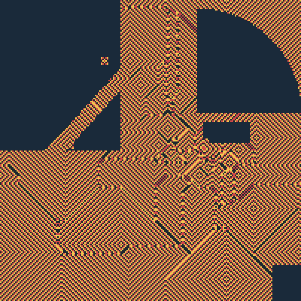
Visual asset

Primary: assets/tokyo_ca_voronoi_t160.png (200 × 200 → 600 × 600 upscaled, NEAREST). Yellow-orange checkerboard texture is the oscillating excitable medium; bright yellow ridges across the field are wave-front collision lines = Voronoi edges between food cells. Central diamond pattern = waves converging from the Tokyo cluster. Dark-blue regions are inert mask (Pacific, Tokyo Bay, mountains).

Time series (also in assets/): tokyo_ca_t030.png, tokyo_ca_t060.png, tokyo_ca_t100.png — show convergence progression for the slide’s mid-presentation animation.

References (per Tut, foundation lane)

Greenberg, J.M. and Hastings, S.P. (1978). "Spatial patterns for
discrete models of diffusion in excitable media." SIAM J. Appl.
Math. 34(3), 515-523.
— origin of the 3-state excitable CA rule we run.

Tolmachev, D. and Adamatzky, A. (1996). "Chemical processor for
computation of Voronoi diagram." Adv. Mater. Optics Electron. 6(4),
191-196.
— wave-front collision on excitable media computes Voronoi as a
by-product. Direct precedent for what Tokyo demo shows.

Adamatzky, A. (2010). Game of Life Cellular Automata. Springer.
— Ch. 17 covers maze-solving / Voronoi-computing CA class. Our
Tokyo CA is in this lineage, NOT Tero 2010.

Murray, J.D. (2003). Mathematical Biology II. Springer, 3rd ed.
Chs. 1, 8-10. — accessible textbook treatment of excitable media
for the architect-grade audience.

Molloy, M. and Salavatipour, M.R. (2005). "A bound on the chromatic
number of the square of a planar graph." J. Combin. Theory B 94(2),
189-213. — distance-2 chromatic number 7 of the squared hex lattice;
underwrites the 7-coloring parallel dispatch.

What’s overclaim risk

(Pulled from one_pager.md for completeness.)

“Tokyo CA runs slime mold on the substrate” — wrong. Substrate has no fluid dynamics; engine source explicitly says “No scent diffusion. No fluid dynamics.” Engine docstring is the source of truth. What the Tokyo demo actually shows is a Greenberg-Hastings excitable cellular automaton producing a Voronoi tessellation between food sources, NOT a slime-mold network. Real CA, real convergence, real visualization — but not what Tero 2010 produced biologically.

The mold_walk side demo sits next to this slide on the deck and shows what actually trying for slime mold looks like — on a different substrate, explicitly labelled as Metal-side (see slides/mold_walk_side_demo.md).

Source material

• DagDB engine repo: https://github.com/norayr-m/dagdb-engine
• Tokyo CA test source: dagdb/Tests/DagDBTests/TokyoCATests.swift (testTokyoSolve200x200 — convergence at tick 160, 4.6 s wall)
• Dashboard build scripts: dagdb/examples/tokyo_ca/build_dashboard_data.py + build_dashboard_html.py
• Mold_walk sister substrate (Metal-side, separate repo): ~/000_AI_Work/0_Projects/0_Active_MoldWalk/ (referenced by side demo, not the DagDB run)

Status

Tokyo CA live demo: IN PROGRESS (status board at README.md). - [x] Demo run plan + technical encoding consolidated (demos/tokyo_ca.md) - [x] This slide drafted - [x] UMA performance slide drafted (uma_performance.md) - [x] Visual asset inlined (tokyo_ca_voronoi_t160.png) - [x] GH-link footer added - [ ] Side mold_walk slide (tomorrow afternoon) - [ ] Convergence GIF capture under assets/ - [ ] Pub-screen pass on the GH footer addition

bzz. — slvr.

Layer 3 — Full inventory walk

Calibration: this is the clickable detail behind every direction in Layers 1 and 2. White papers, live demos, repositories, demo scripts, math papers, media. Maintained as new work lands; post-recording this section migrates to the GitHub Profile README as the live wiki end-state.

What

Six categories. Every row links to a real public artefact.

The narration walks the structure; this slide carries the URLs you click.

a) White papers

Five more queued (Decoder, Pipeline, Interstellar, Orbital, Encoder Brain). Engine substrate paper held for explicit trigger.

b) Live demos (browser-runnable)

DagDB family: engine landing · SQL architecture · grid demo · podcast · interview · wiki

Savanna family: interactive presentation · 7-coloring · 1B cell playback · Morton charts · about

Bio digital twin: brain-tile prototype

DRT-X canonical 5-collection: Composer · Scanner · Pipeline · Cell Simulator · Bio D Twin · plus Generator presentation deck

DRT-X standalones: Decoder of the Encoder · Interstellar Harmony · Orbital Solver · Encoder Brain

Other public: Three Basket Backup · Ternary Lattice · Isomorphic Walk viewers

Twenty-five browser-runnable demos at recording time.

c) Repositories

Thirteen active public repositories, plus the Profile.

dagdb-engine · savanna-engine · isomorphic-walk · drt-generator · drt-scanner · drt-cell-simulator · decoder-of-the-encoder · DRT-Encoder-Brain · drt-pipeline · drt-orbital-solver · interstellar-harmony · three-basket-backup · ternary-lattice

Profile: github.com/norayr-m

d) Demo scripts (in flight)

Five scripts in flight: demo order narrative, BACK_EDGE / AC-3 live demo, Tokyo CA on DagDB, honey-on-DagDB, tile-streaming spec walkthrough.

e) Math papers (referenced)

Distributed Reconstruction Theorem v0.1 — in preparation.

Ternary firewall topological regularization (CVPDE) — in preparation, separate venue, not the focus of this work.

f) Media

YouTube: Savanna v0.6 · Swift Infection · Swift Haboob · 100B Cell test

Podcasts: DagDB Podcast (Carlos persona) · DagDB Dialogue (same site) · DRT Generator presentation deck narration (embedded)

Interviews: DagDB Podcast Interview

Maintenance discipline

This inventory updates in the same push that lands the work. No separate sync step. Eight-category screen runs every time. Post-recording the structure migrates to the Profile README as the live wiki end-state.

Slot owner: tut (explanatory framing on the inventory walk). Source-of-truth: tier3_inventory.md. Calibration source: one_pager.md.

Active public repos and Profile: github.com/norayr-m.

Q&A — direct questions to specific specialists

Live segment. Each specialist is active in their own tmux session during the Zoom and answers in their own voice via the live audio pipeline.

Format

Direct your question to a specific specialist by name. Norayr relays. The specialist answers on the fly through the live voice pipeline — their actual voice, their actual lane, real-time.

The deck’s multi-voice narration is the rehearsal; the Q&A is the live demonstration.

Specialists available — by lane

How to ask

Name the specialist + the question. Norayr passes it to the specialist’s session; their answer lands in audio within seconds.

If you’re unsure which specialist owns a question, name the topic and Norayr routes.

What we will not answer

• Anything outside the calibration anchor (one_pager.md). If a specialist doesn’t have verified-or-spec material on a topic, the answer will say so explicitly.

The discipline is the same as the deck’s: show what the work IS — name what it isn’t only when directly asked.

Calibration

This Q&A operates under the same calibration discipline as the deck. Every answer maps to verified, spec, or overclaim-risk per one_pager.md. Specialists self-label their answers at the appropriate tier.

If a specialist hits a question outside their lane, they hand off cleanly: “That’s [other-specialist]’s lane — [name], over to you?”

Slot owner: tut (explanatory framing on the section). Live-event ownership: pub (production), varpet (tmux infrastructure), each specialist (their own answers). Calibration source: one_pager.md. Engine source authoritative.

Active public repos — DagDB · Savanna · Isomorphic Walk · drt-generator · drt-scanner · drt-cell-simulator · drt-pipeline · drt-orbital-solver · decoder-of-the-encoder · DRT-Encoder-Brain · interstellar-harmony · three-basket-backup · ternary-lattice. Profile: github.com/norayr-m.